Canalization of the evolutionary trajectory of the
human influenza virus
Trevor Bedford1,2,†,*, Andrew Rambaut3,4 & Mercedes Pascual1,2
1Department of Ecology and Evolutionary Biology, University of Michigan, Ann Arbor, MI, USA.
2Howard Hughes Medical Institute, University of Michigan, Ann Arbor, MI, USA.
3Institute of Evolutionary Biology, University of Edinburgh, Edinburgh, UK.
4Fogarty International Center, National Institutes of Health, Bethesda, MD, USA.
†Present address: Institute of Evolutionary Biology, University of Edinburgh, Edinburgh, UK.
*Correspondence: t.bedford@ed.ac.uk
Citation
Bedford T, Rambaut A, Pascual M. 2012. Canalization of the evolutionary trajectory of the
human influenza virus. BMC Biol 10: 38.
Abstract
Background: Since its emergence in 1968, influenza A (H3N2) has evolved extensively in
genotype and antigenic phenotype. However, despite strong pressure to evolve away from human
immunity and to diversify in antigenic phenotype, H3N2 influenza shows paradoxically limited
genetic and antigenic diversity present at any one time. Here, we propose a simple
model of antigenic evolution in the influenza virus that accounts for this apparent
discrepancy.
Results: In this model, antigenic phenotype is represented by a N-dimensional vector and virus
mutations perturb phenotype within this continuous Euclidean space. We implement this
model in a large-scale individual-based simulation, and in doing so, find a remarkable
correspondence between model behavior and observed influenza dynamics. This model
displays rapid evolution but low standing diversity and simultaneously accounts for the
epidemiological, genetic, antigenic and geographical patterns displayed by the virus. We find that
evolution away from existing human immunity results in rapid population turnover in the
influenza virus and that this population turnover occurs primarily along a single antigenic
axis.
Conclusions: Selective dynamics induce a canalized evolutionary trajectory, in which the
evolutionary fate of the influenza population is surprisingly repeatable. In the model, the
influenza population shows a 1–2 year timescale of repeatability, suggesting a window in which
evolutionary dynamics could be, in theory, predictable.
Abstract
Introduction
Epidemic influenza is responsible for between 250,000 and 500,000 global deaths annually, with
influenza A (and in particular, A/H3N2) having caused the bulk of human mortality and
morbidity [1]. Influenza A (H3N2) has continually circulated within the human population since
its introduction in 1968, exhibiting recurrent seasonal epidemics in temperate regions and less
periodic transmission in the tropics. During this time, H3N2 influenza has continually evolved
both genetically and antigenically. Most antigenic drift is thought to be driven by
changes to epitopes in the hemagglutinin (HA) protein [2]. Phylogenetic analysis of
the relationships among HA sequences has revealed a distinctive genealogical tree
showing a single predominant trunk lineage and side branches that persist for only 1–5
years before going extinct [3]. This tree shape is indicative of serial replacement of
strains over time; H3N2 influenza shows rapid evolution, but low standing genetic
diversity.
This observation has remained puzzling from an epidemiological standpoint. Antigenic evolution
occurs rapidly and strong diversifying selection exists to escape from human immunity; why then
do we see serial replacement of strains rather than continual genetic and antigenic diversification?
Indeed, simple epidemiological models show explosive diversity of genotype and phenotype
over time [4, 5]. Previous work has sought model-based explanations of the limited
diversity of influenza, relying on short-lived strain-transcending immunity [4, 5],
complex genotype-to-phenotype maps [6] or a limited repertoire of antigenic phenotypes
[7].
Experimental characterization of antigenic phenotype is possible through the hemagglutination
inhibition (HI) assay, which measures the cross-reactivity of HA from one virus strain to serum
raised against another strain [8]. The results of many HI assays can be combined to
yield a two-dimensional map, representing antigenic similarity and distance between
strains as an easily visualized and quantified measure [9]. The path traced across this
map by influenza A (H3N2) from 1968 until present is largely linear, showing serial
replacement of one strain by another; there are no major bifurcations of antigenic phenotype
[9].
Herein, we seek to simultaneously model the genetic and antigenic evolution of the
influenza virus. We represent antigenic phenotypes as points in a N-dimensional Euclidean
space. Based on the finding that a two-dimensional map adequately explains observed
antigenic distance between strains [9], we begin with antigenic phenotypes as points
on a plane, but relax this assumption later on in the analysis. After exposure to a
virus, a host’s risk of infection is proportional to the Euclidean distance between the
infecting phenotype and the closest phenotype in the host’s immune history. Mutations
perturb antigenic phenotype, moving phenotype in a random radial direction and for a
randomly distributed distance. We implemented this geometrical model in a large-scale
individual-based simulation intended to directly model the antigenic map and genealogical tree of
the global influenza population. The simulation includes multiple host populations
with different seasonal forcing, hosts with complete immune histories of infection, and
viruses with antigenic phenotypes. As the simulation proceeds, infections are tracked
and a complete genealogy connecting virus samples is constructed. Results shown
here are for simulations of 40 years of virus evolution in a population of 90 million
hosts.
Results and Discussion
Antigenic evolution and genealogical patterns
The virus persists over the course of the 40-year simulation, and at the end of most simulations,
there remain only a few closely related viral lineages, indicating that genealogical diversity is
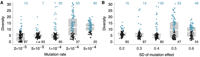
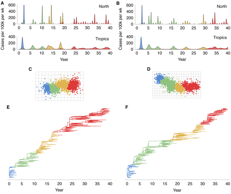
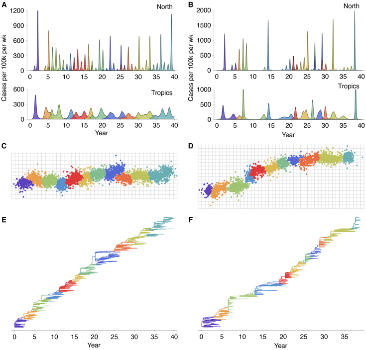
restricted by evolution in the two-dimensional antigenic landscape. Reduced diversity is
substantially more common in models with less mutation or models with less variable
mutation effects (Figure 1). At higher mutation rates, viruses may move apart in
antigenic phenotype too rapidly for competition to always eliminate the weaker of two
diverging lineages. Similarly, with high variance in mutational effect, there can sometimes
emerge new antigenic types, too distant from the existing population to suffer limiting
competitive pressure. Both these scenarios lead to coexistence of multiple antigenic
phenotypes. We thus restrict the model to parameter regimes with lower mutation rates and
lower mutation effect variances. We primarily focus on the model with 10-4 mutations
per infection per day and mutation effects with standard deviation of 0.4 antigenic
units. In this model, 80 out of the 100 replicate simulations show reduced genealogical
diversity (defined as less than 9 years of evolution separating contemporaneous viruses).
We conditioned the following analysis on these 80 simulations, compiling summary
statistics across this pool and presenting a detailed analysis of a single representative
simulation.
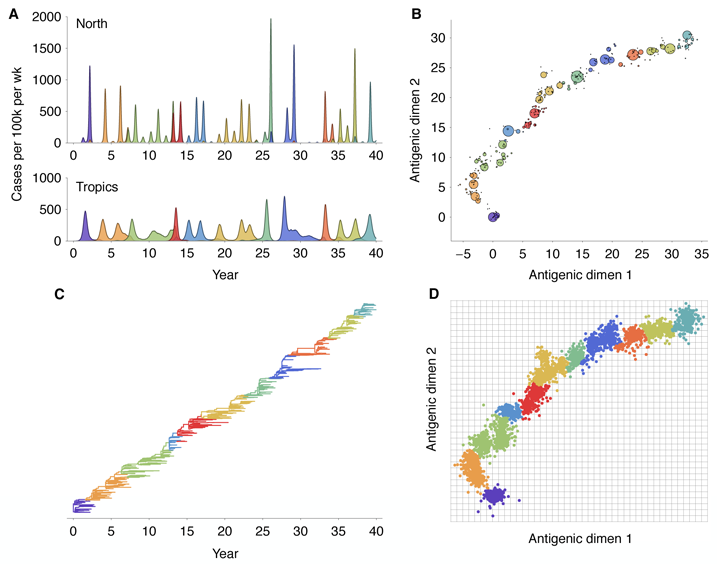
The model exhibits annual winter epidemics in temperate regions and less periodic epidemics in
the tropics (Figure 2A). Across replicate simulations, we observe average yearly attack rates of
6.8% in temperate regions and rates of 7.1% in the tropics, comparable with estimated
attack rates of influenza A (H3N2) of 3–8% per year [10, 11]. Over the course of the
simulation, the virus population evolves in antigenic phenotype exhibiting, at any point, a
handful of highly abundant phenotypes sampled repeatedly and a large number of
phenotypes appearing at low abundance (Figure 2B). The observed antigenic map of
H3N2 influenza includes substantial experimental noise; replicate strains appear in
diverse positions on the observed map. By including measurement noise on antigenic
locations (see Methods), we approximate an experimental antigenic map of H3N2
influenza (Figure 2D). Over the 40-year simulation, antigenic drift moves the virus
population at an average rate across replicate simulations of 1.05 antigenic units per year,
corresponding closely to the empirical rate of 1.2 units per year [9]. The appearance
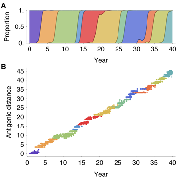
of clusters in the antigenic map comes from the regular spacing of high abundance
phenotypes combined with measurement noise. Over time, clusters of antigenically
similar strains are replaced by novel clusters of more advanced strains (Figure 3A).
Across replicate simulations, clusters persist for an average of 5.0 years, measured as
the time it takes for a new cluster to reach 10% frequency, peak and decline to 10%
frequency. The transition between clusters occurs quickly, taking an average of 1.8
years.
Remarkably, although antigenic phenotype is free to mutate in any direction in the
two-dimensional space, selection pressures force the virus population to move in nearly a straight
line in antigenic space (Figure 2B). Across replicate simulations, 94% of the variance of antigenic
phenotype can be explained by a single dimension of variation. This mirrors the empirical results
showing a largely linear antigenic map for H3N2 influenza isolates from 1968 to 2003 [9].
Because of the primarily one-dimensional movement, antigenic distance from the original
phenotype increases nearly linearly with time (Figure 3B). Antigenic evolution occurs in a
punctuated fashion; periods of relative stasis are interspersed with more rapid antigenic
change (Figure 3B). Antigenic and epidemiological dynamics show a fundamental
linkage, so that large jumps of antigenic phenotype result in increased rates of infection
(Figure 2).
The genealogical tree connecting the evolving virus population appears characteristically sparse
with pronounced trunk and short-lived side branches (Figure 2C). This tree shape is reflected in
low levels of standing diversity; across replicates, an average of 5.68 years of evolution separate
two randomly sampled viruses in the population. This result matches well with the average
diversity observed in influenza A (H3N2) of 5.65 years separating randomly sampled
contemporaneous viruses [12]. A spindly genealogical tree is indicative of population turnover,
wherein novel antigenic phenotypes continually replace more primitive ‘spent’ phenotypes,
purging their genealogical diversity. In general, natural selection reduces effective population size
and genealogical diversity [12].
Selective pressures can be examined by comparing which mutations fix, i.e. are incorporated into
the progenitor trunk lineage, and which mutations are lost, i.e. incorporated into side
branches bound for extinction. This approach has shown that, in influenza A (H3N2),
natural selection promotes mutations to epitope sites in the HA1 region [13, 14]. By
examining antigenic mutations, we find a corresponding effect in simulated evolutionary
trajectories (Table 1). Additionally, we find that trunk mutations occur at strikingly
regular intervals, with less variation of waiting times than expected under a simple
random process (Figure 4). There is a relative scarcity of mutation events occurring in
intervals under 1 year and a relative excess of a mutation events occurring in 2–3 year
intervals (Figure 4). This pattern arises from clonal interference between competing
mutations which reduces variability in the fixation process of adaptive substitutions
[15].
Table 1: Rates of mutation and phenotypic change on trunk and side branches
and mutational expectation.
|
|
|
|
|
| | Baseline | Side branch | Trunk | Trunk / side branch |
|
|
|
|
|
| Mutation size (AG units) | 0.60 | 0.79 | 1.58 | 1.99× |
| Mutation rate (mut per year) | 0.04 | 0.06 | 0.81 | 13.23× |
| Antigenic flux (AG units per year) | 0.02 | 0.05 | 1.27 | 26.25× |
|
|
|
|
|
| |
Spatial dynamics
The genealogical tree also contains detailed information on the history of migration between
regions. We find that, consistent with empirical estimates [16, 17], the trunk resides primarily
within the tropics, where seasonal dynamics are less prevalent (Figure 5A). Across replicate
simulations, we observe 72% of the trunk’s history within the tropics and 28% within temperate
regions. With symmetric host contact rates and equal host population sizes, and without
seasonal forcing, we would expect trunk proportions of one third for each region. We
calculated rates of migration based on observed event counts across replicate simulations,
separating region-specific rates on side branches from region-specific rates on trunk
branches. We find that migration patterns on side branches are close to symmetric,
with similar rates between all regions, while migration patterns on trunk branches are
highly asymmetric, with high rates of movement between temperate regions and from
temperate regions into the tropics (Figure 5B). Extrapolating from these rates, we
arrive at an expected stationary distribution of trunk location of 76% tropics and 24%
temperate regions, in line with the observed residency patterns of the trunk. It may at first
seem counter-intuitive to see higher rates of movement from the temperate regions
into the tropics along trunk branches, but it makes sense when thought of in terms of
conditional probability. Only those lineages that remain in the tropics, migrate into
the tropics or which rapidly migrate between the north and south have a chance at
becoming the trunk lineage, while lineages that remain within the temperate regions are
doomed to extinction. Along similar lines, Adams and McHardy [18] use a modeling
approach to show the importance of non-seasonal transmission to the evolution of the
virus.
These findings suggest that persistence and migration are fundamentally connected and have
important implications for future phylogeographic analyses. Russell et al. [16] emphasize a
source-sink model of movement of the HA protein of influenza A (H3N2) based on
their finding of a trunk lineage residing within China and the Southeast Asian tropics.
Whereas, Bedford et al. [17] emphasize a global metapopulation model based on
phylogenetic inference of migration rates across the entire tree. Our results suggest that both
scenarios are simultaneously possible; side branches may be highly volatile moving
rapidly and symmetrically between regions, while the trunk lineage may be more stable
remaining within a region (or within a highly connected network of regions) that has more
persistent transmission. In light of these results, we suggest that future work on the
phylogeography of influenza take into account trunk vs. side branch differences in migration
patterns.
Correspondence between model and data
In our model, antigenic evolution is driven by the appearance of novel antigenic variants that best
escape existing human immunity. Although multiple epidemiological/evolutionary mechanisms
have been proposed to explain the restricted genetic diversity and rapid population
turnover of influenza A (H3N2) [4, 5, 6, 7], our results show that a simple model
coupling antigenic and genealogical evolution exhibits broad explanatory power. We find a
strong correspondence between the antigenic and genealogical patterns generated by
our model (Figure 2) and patterns of genetic and antigenic evolution exhibited by
influenza A (H3N2) [3, 9]. Our model simultaneously captures seasonal attack rates, the
rate and pattern of antigenic drift, genealogical diversity and geographic migration
patterns.
Our model predicts that detailed classification of influenza strains will support a relatively small
number of predominant phenotypes. Rather than each influenza strain possessing a unique
antigenic location, many strains group together with shared antigenic phenotypes (Figure 2B).
We suggest that a large proportion of intra-cluster variation in the observed antigenic map is due
to experimental noise, rather than each strain possessing a unique antigenic location. The
relationship between Figure 2B and Figure 2D illustrates this effect, where a large number of
antigenic locations emerge from a comparatively small number of unique antigenic
phenotypes. Additionally, our model accurately predicts the contrasting dynamics of other
types/subtypes of influenza. We find that lowering mutation size/effect or lowering
intrinsic R0 results in decreased incidence, slower antigenic movement and greater
genealogical diversity, all distinguishing characteristics of H1N1 influenza and influenza B
(Figure S1).
The historical record of influenza evolution suggests that bifurcation of viral lineages is rare, but
possible. We have observed no bifurcations in H1N1 influenza from 1918 to 1957 and again from
1977 to 2010, no bifurcations in H2N2 influenza from 1957 to 1968 and no bifurcations of H3N2
influenza from 1968 to 2010. We have observed one bifurcation in influenza B from 1980 to 2010.
Thus, ignoring differences between influenza types and subtypes, we have very roughly observed a
rate of one major bifurcation in 155 years of evolution. In our model, in 20 out of 100 replicate
simulations, we observe a deep bifurcation in the viral genealogy, which translates to observing
one deep bifurcation in 200 years of evolution. Thus, we suggest that the 20 of 100
simulations where deep branching occurs are not necessarily evidence of poor model
fit. Similar to Koelle et al. [19], we assume that although the historical evolution of
H3N2 influenza followed the path of a single lineage, it could have included a major
bifurcation.
In our model, when antigenic phenotype remains static, there may be multiple consecutive
seasons without appreciable incidence (Figure 2A), a pattern apparently absent from H3N2
influenza [20]. Additionally, we observe antigenic trajectories that are more linear and
deterministic than the highly clustered trajectory observed by Smith et al. [9]. We suggest that
any model exhibiting punctuated evolution broadly consistent with the punctuated change seen
in the experimental antigenic map will show similar patterns of incidence. We can ‘fix’ the
incidence patterns, but at the cost of too smooth an antigenic map (Figure S2). Evolutionary
patterns of the neuraminidase (NA) protein may provide an explanation. Epitopes in the HA and
NA proteins are jointly responsible for determining antigenicity [2], and it is now clear that
levels of adaptive evolution are similar between HA and NA [21]. Thus, changes in
NA may be driving incidence patterns as well, resulting in an observed timeseries of
incidence partially divorced from the antigenic map of HA. Incorporating antigenic
evolution of NA could thus yield a rougher antigenic map for HA, more closely matching
experimental results, while simultaneously yielding smoother year-to-year incidence
patterns.
It remains a central question as to the extent that short-lived strain-transcending immunity is
responsible for influenza’s limited diversity and spindly genealogical tree [4, 5]. Our findings
suggest a possible resolution. Although lacking short-lived immunity, our model shows a detailed
correspondence to both the antigenic map and genealogical tree of H3N2 influenza. If an
antigenic map were to show a deep bifurcation, where two viral lineages move in different
antigenic directions, then we would expect the same bifurcation to be evident in the genealogical
tree. Short-lived strain-transcending immunity provides a mechanism by which lineages may
diverge in antigenic phenotype, but still show epidemiological interference. This mechanism would
explain a situation where bifurcations emerge in the antigenic map, but competition results
in the extinction of divergent antigenic lineages. In our model, one cluster leads to
another cluster in orderly succession and there is never competition between antigenically
distant clusters. Thus, short-lived strain-transcending immunity is not required to
limit diversity in the model. This is not to say that short-lived strain-transcending
immunity is not present; observed interference between subtypes [4, 22], evolution at CTL
epitopes [23] and the exclusion of the Beijing/89 cluster by the antigenically distant
Beijing/92 cluster [9] all suggest some form of more general interaction between influenza
viruses.
Linear antigenic movement
It might seem reasonable for one viral lineage to move in one antigenic direction, while another
lineage moves tangentially, eventually resulting in two non-interacting viral lineages. Instead, we
find that movement in a single antigenic direction is favored, resulting in most replicate
simulations showing low standing diversity (Figure 1). The origins of this pattern can be seen in
the interaction between virus evolution and host immunity (Figure 6). As the virus population
evolves forward it leaves a wake of immunity in the host population, and evolution away from this
immunity results in the canalization of the antigenic phenotype; mutations that continue along
the line of primary antigenic variation will show a transmission advantage compared to more
tangential mutations.
Following the work of Smith et al. [9], it remained an open question of why a two-dimensional
map should explain the antigenic variation of H3N2 influenza. Although the authors astutely
speculated that “there is a selective advantage for clusters that move away linearly from previous
clusters as they most effectively escape existing population-level immunity, and this is a plausible
explanation for the somewhat linear antigenic evolution in regions of the antigenic map.” This
hypothesis remained to be tested. Here, we show from a simple model of epidemiology and
evolution that a linear trajectory of antigenic evolution dynamically emerges due to basic
selective pressures. This result simultaneously explains the linear pattern of antigenic drift
[9] and the characteristically spindly genealogical tree [3] exhibited by influenza A
(H3N2).
For this process to take hold, the virus population needs to be somewhat mutationally-limited; if
functional antigenic variants of novel phenotype emerge too quickly, then antigenic change will
occur too rapidly for competition to winnow down the virus population to a single lineage
(Figure 1). Assuming that antigenic mutations have an average effect of 0.6 antigenic
units and a standard deviation of 0.4 units, then the rate of new antigenic mutations
cannot be greater than approximately 10-4 mutations per day (Figure 1). Thus, it is
important that the rate of 10-4 mutations per day be biological plausible. Here, we
take the rate of synonymous substitution as a proxy for the neutral rate of mutation.
The rate of synonymous change has been estimated at 2.5 × 10⁻⁶ per site per day
[24]. As there are approximately 2 nonsynonymous sites per codon in influenza [25],
this gives a neutral rate of amino acid change of approximately 5 × 10⁻⁶ per site per
day. Other work has shown that there appear to be ~18 amino acid sites implicated
in the majority of adaptive change [13]. These sites evolve along the trunk of the
phylogeny at rate of 0.053 substitutions per site per year or at a combined rate of 0.95
substitutions per year [4]. This result agrees well with our finding of 0.81 antigenic
mutations per year on the phylogeny trunk (Table 1). If we assume 18 sites involved in
antigenic change, this gives an overall rate of antigenic mutation of 9 × 10⁻⁵ per day.
Thus, we believe that 10-4 mutations per day represents a biologically reasonable
estimate.
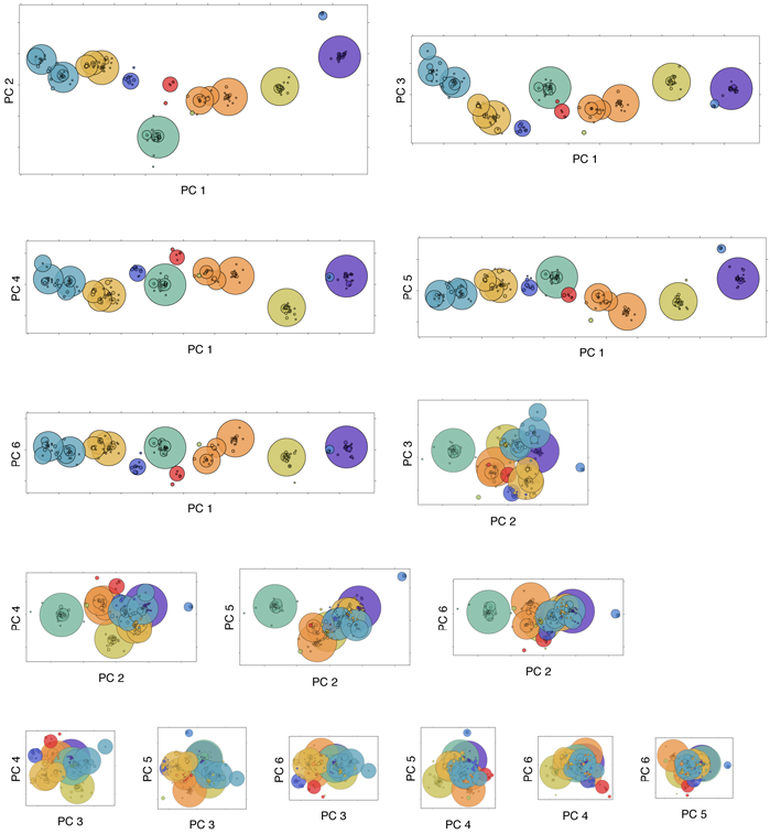
To consider to what extent these results were contingent on the dimensionality of the
underlying antigenic model, we further implemented our model in a 10-dimensional
antigenic space. Here, mutations occur as 10-spheres, but the distance moved by a
mutation is the same as in the previous two-dimensional formulation. We arrive at nearly
the same results with this model; principal components analysis shows that the first
and second dimensions of variation account for 87% and 7%, respectively, of the total
variance (Figure S3). Thus, our model predicts that future work probing mutational
effects will support an underlying high-dimensional antigenic space, even though a
two-dimensional map is sufficient to explain observed antigenic relationships among evolving
strains.
Winding back the tape
The 40-year simulation of influenza dynamics shows broad correspondence with observed
patterns. However, year-to-year details are not captured, e.g. years that undergo antigenic
transitions in the 40-year simulation do not match up with observed years of antigenic
transitions. Over long time spans, year-to-year correspondence seems impossible to achieve in this
sort of stochastic system, where evolution is often driven by chance mutations of large antigenic
effect. However, correspondence in the shorter term may be possible. To test this, we examined
repeatability in replicate simulations, showing what happens when we “wind back
the tape” [26] on the evolution of the virus. We ran 100 replicate simulations, each
starting from the endpoint of the representative 40-year simulation shown in Figure
2. The starting point for these replicate simulations was the exact end state of the
40-year simulation, including the frequencies of every virus strain and the entire host
immune profile. These replicate simulations were run for an additional 6 years, and
all evolutionary and epidemiological parameters were identical to the initial 40-year
simulation.
Initially, we find a great detail of repeatability; during the first year of evolution, every replicate
virus population undergoes a similar antigenic transition (Figure 7), resulting in a repeatable
peak in northern hemisphere incidence (Figure 8). After three years, repeatability has mostly
disappeared, with antigenic phenotype and incidence appearing highly variable across replicates
(Figure 7, Figure 8). The 1–2 year timescale of repeatability can be explained by the presence of
standing antigenic variation. In the initial virus population, there are several novel antigenic
variants present at low frequency (Figure 6), one of which, without fail, comes to predominate
the virus population.
We see that the initial evolutionary trajectory, during which time standing variation plays out, is
highly repeatable, and thus predictable given enough information and the right methods of
analysis. However, prediction of longer-term evolutionary scenarios will necessarily be difficult or
impossible except in a vague sense. Through careful surveillance efforts and genetic and antigenic
characterization of influenza strains, the World Health Organization makes twice-yearly vaccine
strain recommendations [27]. It should be possible to combine these sorts of modeling
approaches with surveillance data to gauge the likelihood that a sampled variant will spread
through the population.
Conclusions
Recent work on empirical fitness landscapes has shown that natural selection follows few
mutational paths [28]. The spindly genealogical tree and the almost linear serial replacement of
influenza strains has remained a puzzling phenomenon. We suggest that the evolutionary and
epidemiological dynamics displayed by the influenza virus may simply be explained as an
outgrowth of selection to avoid host immunity. Natural selection can only ‘see’ one step ahead,
and so sacrifices long-term gains for short-term advantages. The result is a canalized evolutionary
trajectory lacking antigenic diversification.
Methods
Transmission model
To characterize the joint epidemiological, genealogical, antigenic and spatial patterns of influenza,
we implemented a large-scale individual-based model (full simulation source code available at
http://www.trevorbedford.com/antigen/). This model consists of daily time steps,
in which the states of hosts and viruses are updated. Hosts may be born, may die,
may contact other hosts allowing viral transmission, or may recover from infection.
Viruses may mutate in antigenic phenotype. Each simulation ran for 40 years of model
time.
Hosts in this model are divided between three regions: North, South and Tropics. There are 30
million hosts within each of the three regions, giving N = 9 × 10⁷ hosts. Host population size
remains fixed at this number, but vital dynamics cause births and deaths of hosts at a rate of
1∕30 years = 9.1 × 10⁻⁵ per host per day. Within each region, transmission proceeds through
mass-action with contacts between hosts occurring at a rate of β = 0.36 per host per day.
Regional transmission rates in temperate regions vary according to sinusoidal seasonal forcing
with amplitude ϵ = 0.15 and opposite phase in the North and in the South. Transmission rate
does not vary over time in the Tropics. Transmission between region i and region j
occurs at rate mβi, where m = 0.001 and is the same between each pair of regions and
βi is the within-region contact rate. Hosts recover from infection at rate ν = 0.2 per
host per day, so that R0 in a naive host population is 1.8. An individual cannot be
simultaneously infected with multiple virus lineages; there is no super-infection in the
model.
Each virus possesses an antigenic phenotype, represented as a location in Euclidean space. Here,
we primarily use a two-dimensional antigenic location. After recovery, a host ‘remembers’ the
phenotype of its infecting virus as part of its immune history. When a contact event occurs and a
virus attempts to infect a host, the Euclidean distance from infecting phenotype ϕv is calculated
to each of the phenotypes in the host immune history ϕh1,…,ϕhn. Here, one unit of
antigenic distance is designed to correspond to a twofold dilution of antiserum in a
hemagglutination inhibition (HI) assay [9]. The probability that infection occurs after exposure
is proportional to the distance d to the closest phenotype in the host immune history. Risk of
infection follows the form ρ = min{ds,1}, where s = 0.07. Cross-immunity σ equals
1 - ρ. With no initial immunity in the host population, the virus undergoes a severe
trough in prevalence after the initial pandemic increase. With this number of host
individuals, the virus population usually stochastically dies out during this trough. To
prevent this, we gave the initial host population enough immunity to slow down the
initial virus upswing and place the dynamics closer to their equilibrium state; initial R
was 1.28. Future work should attempt to more accurately model initial evolutionary
dynamics.
As in the current analysis, previous studies [4, 6, 7], have assumed that host immune response
is dictated by the closest phenotype in the immune history. Due to original antigenic sin, other
phenotypes in the host immune history may have a disproportionate effect on host immunity.
This may be an important aspect to modeling influenza, and should be addressed in future
studies. Our model follows Lin et al. [29] and Gog and Grenfell [30] in representing antigenic
distance as distance between points in a geometric space. By forcing one-dimension to directly
modulate β, Gog and Grenfell find an orderly replacement of strains. Kryazhimskiy et al. [31]
use a two-dimensional strain-space, in which cross-immunity between two strains is
proportional to their distance in one or dimension or the other, whichever is closer. This
cross-immunity kernel directly favors moving along a diagonal line away from previous
strains. Our model more closely approximates how HI distance is incorporated into
the Smith et al. [9] antigenic map; HI between strains is projected as a Euclidean
distance, rather than as the closest distance between strains in either dimension one or
two.
The initial virus population consisted of 10 infections each with the identical antigenic phenotype
of {0,0}. Over time viruses evolve in antigenic phenotype. Each day there is a chance μ = 10-4
that an infection mutates to a new phenotype. This mutation rate represents a phenotypic rate,
rather than genetic mutation rate, and can be thought of as arising from multiple genetic sources.
When a mutation occurs, the virus’s phenotype is moved in a completely random direction
~ Uniform(0,360) degrees. Mutation size is sampled from the distribution ~ Gamma(α,β), where
α and β are chosen to give a mean mutation size of δavg = 0.6 units and a standard
deviation of δsd = 0.4 units. This distribution is parameterized so that mutation usually
has little effect on antigenic phenotype, but occasionally has a larger effect. This is
similar to the neutral networks implemented by Koelle et al. [6], wherein most amino
acid changes result in little decrease to cross-immunity between strains, but some
changes result in large jumps in cross-immunity. This mutation model implicitly assumes
independence between mutations; each mutation’s effect is independent of genetic
background.
Model output
Daily incidence and prevalence are recorded for each region. During the course of the simulation,
samples of current infections are taken from the evolving virus population at a rate proportional
to prevalence. Each viral infection is assigned a unique ID, and in addition, infections have their
phenotypes, locations and dates of infection recorded. In this model, viruses lack sequences and
so standard phylogenetic inference of the evolutionary relationships among strains is impossible.
Instead, the viral genealogy is directly recorded. This is made possible by tracking transmission
events connecting infections during the simulation; infections record the ID of their ‘parent’
infection. Proceeding from a sample of infections, their genealogical history can be
reconstructed by following consecutive links to parental infections. Following this procedure,
lineages coalesce to the ancestral lineages shared by the sampled infections, eventually
arriving at the initial infection introduced at the beginning of the simulation. Commonly,
phylodynamic simulations generate sequences that are subsequently analyzed with
phylogenetic software to produce an estimated genealogy [4, 6, 32]. This step of
phylogenetic inference is imperfect and computationally intensive, and by side-stepping
phylogenetic reconstruction we arrive at genealogies quickly and accurately. Other authors
have implemented similar tracking of infection trees [33, 34]. This genealogy-centric
approach makes many otherwise difficult calculations transparent, such as calculating
lineage-specific region-specific migration rates (Figure 5) and lineage-specific mutation effects
(Table 1).
Infections are sampled at a rate designed to give approximately 6000 samples over the course of
the simulation, with genealogies constructed from a subsample of approximately 300 samples.
The results presented in Figure 2 represent a single representative model output; one hundred
replicate simulations were conducted to arrive at statistical estimates.
Parameter selection and sensitivity analysis
Estimating what the basic reproductive number R0 for seasonal influenza would be in a naive
population is notoriously difficult. Season-to-season estimates of effective reproductive number R
for the USA and France gathered from mortality timeseries display an interquartile range of
0.9–1.8 [35]. Geographic spread within the USA suggests an average seasonal R of 1.35 [36].
These estimates of R will be lower than the R0 of influenza due to the effects of human immunity.
We assumed R0 of 1.8, consistent with the upper range of seasonal estimates. Duration of
infection was chosen based on patterns of viral shedding shown during challenge studies
[37]. The linear form of the risk of infection and its increase as a function of antigenic
distance s = 0.07 was based on experimental work on equine influenza [38] and from
studies of vaccine effectiveness [39]. Between-region contact rate m was chosen to
yield a trunk lineage that resides predominantly in the tropics. With much higher
rates of mixing, the trunk lineage ceases to show a preference the tropics, and with
much lower rates of mixing, particular seasons in the north and the south will often be
skipped. The amplitude of seasonal forcing ϵ was chosen to be just large enough to get
consistent fade-outs in the summer months and is consistent with empirical estimates
[40].
Mutational parameters were based, in part, on model behavior. We assumed 10 amino acid sites
involved in antigenicity, each mutating at a rate of 10-5 [41] to give a phenotypic mutation rate
μ = 10-4 per infection per day. We chose mutational effect parameters (δavg = 0.6,
δsd = 0.4) that would give suitably fast rates of antigenic evolution corresponding to
approximately 1.2 units of antigenic change per year, while simultaneously giving clustered
patterns of antigenic evolution [9]. Similar outcomes are possible under a variety of
parameterizations. If mutations are more common (μ = 3 × 10⁻⁴) and show less variation in effect
size (δavg = 0.6, δsd = 0.2), then antigenic drift occurs in a more continuous fashion,
resulting in less variation in seasonal incidence and a smoother distribution of antigenic
phenotypes (Figure S2A, C). If mutations are less common (μ = 5 × 10⁻⁵) and show
more variance in effect (δavg = 0.7, δsd = 0.5), then antigenic change occurs in a more
punctuated fashion (Figure S2B, D). Basic reproductive number R0 can be traded off with
mutational parameters to some extent. Less mutational input and higher R0 will give similar
patterns of antigenic drift and seasonal incidence. Similarly, Kucharski and Gog [42]
find that increasing R0 results in increased rates of emergence of antigenically novel
strains.
Antigenic map
Antigenic phenotypes are modeled as discrete entities on the Euclidean plane; multiple samples
have the same antigenic location. However, in the empirical antigenic map of influenza A (H3N2),
each strain appears in a unique location [9]. We would argue that some of this pattern comes
from experimental noise. Indeed, Smith et al. [9] find that observed measurements and
measurements predicted from the map differ by an average of 0.83 antigenic units with a
standard deviation of 0.67 antigenic units. We take this as a proxy for experimental noise and
add jitter to each sampled antigenic phenotype by moving it in a random direction
for an exponentially distributed distance with mean of 0.53 antigenic units. If two
samples with the same underlying antigenic phenotype are jittered in this fashion, the
distance between them averages 0.83 antigenic units with a standard deviation of 0.64
units.
We added noise to each of the 5943 sampled viruses in this fashion resulting in an approximated
antigenic map (Figure 2D). Virus samples were then clustering following standard clustering
algorithms. We tried clustering by the k-means algorithm and also agglomerative hierarchical
clustering with a variety of linkage criterion. We found that clustering by Ward’s criterion
consistently outperformed other methods, when measured in terms of within-cluster and
between-cluster variances. However, the exact clustering algorithm had little effect on our overall
results.
Acknowledgments
We would like to thank Sarah Cobey, Aaron King, Pejman Rohani and the attendees of the 2011
RAPIDD Workshop on Phylodynamics for helpful discussion. We would also like to thank Ed
Baskerville and Daniel Zinder for programming advice. The term ‘canalization’ was originally
suggested by Micaela Martinez-Bakker.
Funding
TB acknowledges support from the European Molecular Biology Organization. AR works as a
part of the Interdisciplinary Centre for Human and Avian Influenza Research (ICHAIR) and the
University of Edinburgh’s Centre for Immunity, Infection and Evolution (CIIE). MP is an
investigator of the Howard Hughes Medical Institute.
References
1. WHO (2009) Influenza Fact sheet. Available at
http://www.who.int/mediacentre/factsheets/fs211/en/.
2. Nelson MI, Holmes EC (2007) The evolution of epidemic influenza. Nat Rev
Genet 8: 196–205.
3. Fitch WM, Bush RM, Bender CA, Cox NJ (1997) Long term trends in the
evolution of H(3) HA1 human influenza type A. Proc Natl Acad Sci USA 94: 7712-8.
4. Ferguson NM, Galvani AP, Bush RM (2003) Ecological and immunological
determinants of influenza evolution. Nature 422: 428–433.
5. Tria F, Lässig M, Peliti L, S F (2005) A minimal stochastic model for influenza
evolution. J Stat Mech .
6. Koelle K, Cobey S, Grenfell B, Pascual M (2006) Epochal evolution shapes
the phylodynamics of interpandemic influenza A (H3N2) in humans. Science 314:
1898–1903.
7. Recker M, Pybus O, Nee S, Gupta S (2007) The generation of influenza outbreaks
by a network of host immune responses against a limited set of antigenic types. Proc
Natl Acad Sci USA 104: 7711–7716.
8. Hirst G (1943) Studies of antigenic differences among strains of influenza A by
means of red cell agglutination. J Exp Med 78: 407–423.
9. Smith DJ, Lapedes AS, de Jong JC, Bestebroer TM, Rimmelzwaan GF, et al.
(2004) Mapping the antigenic and genetic evolution of influenza virus. Science 305:
371–376.
10. Monto A, Sullivan K (1993) Acute respiratory illness in the community.
Frequency of illness and the agents involved. Epidemiol Infect 110: 145–160.
11. Koelle K, Kamradt M, Pascual M (2009) Understanding the dynamics of rapidly
evolving pathogens through modeling the tempo of antigenic change: influenza as a
case study. Epidemics 1: 129–137.
12. Bedford T, Cobey S, Pascual M (2011) Strength and temp of selection revealed
in viral gene genealogies. BMC Evol Biol 11: 220.
13. Bush R, Fitch W, Bender C, Cox N (1999) Positive selection on the H3
hemagglutinin gene of human influenza virus A. Mol Biol Evol 16: 1457–1465.
14. Wolf YI, Viboud C, Holmes EC, Koonin EV, Lipman DJ (2006) Long intervals of
stasis punctuated by bursts of positive selection in the seasonal evolution of influenza
A virus. Biol Direct 1: 34.
15. Park S, Krug J (2007) Clonal interference in large populations. Proc Natl Acad
Sci USA 104: 18135–18140.
16. Russell CA, Jones TC, Barr IG, Cox NJ, Garten RJ, et al. (2008) The global
circulation of seasonal influenza A (H3N2) viruses. Science 320: 340–346.
17. Bedford T, Cobey S, Beerli P, Pascual M (2010) Global migration dynamics
underlie evolution and persistence in human influenza A (H3N2). PLoS Pathog 6:
e1000918.
18. Adams B, McHardy A (2011) The impact of seasonal and year-round transmission
regimes on the evolution of influenza a virus. Proc R Soc B 278: 2249–2256.
19. Koelle K, Ratmann O, Rasmussen D, Pasour V, Mattingly J (2011) A
dimensionless number for understanding the evolutionary dynamics of antigenically
variable rna viruses. Proc R Soc Lond B Biol Sci Advance access.
20. Finkelman B, Viboud C, Koelle K, Ferrari M, Bharti N, et al. (2007) Global
patterns in seasonal activity of influenza A/H3N2, A/H1N1, and B from 1997 to
2005: viral coexistence and latitudinal gradients. PLoS One 2: e1296.
21. Bhatt S, Holmes E, Pybus O (2011) The genomic rate of molecular adaptation
of the human influenza A virus. Mol Biol Evol Advance access.
22. Goldstein E, Cobey S, Takahashi S, Miller J, Lipsitch M (2011) Predicting the
epidemic sizes of influenza A/H1N1, A/H3N2, and B: a statistical method. PLoS
Med In press.
23. Voeten J, Bestebroer T, Nieuwkoop N, Fouchier R, Osterhaus A, et al. (2000)
Antigenic drift in the influenza A virus (H3N2) nucleoprotein and escape from
recognition by cytotoxic T lymphocytes. J Virol 74: 6800–6807.
24. O’Brien J, Minin V, Suchard M (2009) Learning to count: robust estimates for
labeled distances between molecular sequences. Mol Biol Evol 26: 801–814.
25. Yang Z (2000) Maximum likelihood estimation on large phylogenies and analysis
of adaptive evolution in human influenza virus a. Journal of Molecular Evolution 51:
423–432.
26. Gould S (1989) Wonderful life. Norton New York.
27. Barr I, McCauley J, Cox N, Daniels R, Engelhardt O, et al. (2010)
Epidemiological, antigenic and genetic characteristics of seasonal influenza A (H1N1),
A (H3N2) and B influenza viruses: basis for the WHO recommendation on the
composition of influenza vaccines for use in the 2009-2010 Northern Hemisphere
season. Vaccine 28: 1156–1167.
28. Weinreich D, Delaney N, DePristo M, Hartl D (2006) Darwinian evolution can
follow only very few mutational paths to fitter proteins. Science 312: 111–114.
29. Lin J, Andreasen V, Levin S (1999) Dynamics of influenza a drift: the linear
three-strain model. Math Biosci 162: 33–51.
30. Gog J, Grenfell B (2002) Dynamics and selection of many-strain pathogens. Proc
Natl Acad Sci USA 99: 17209–17214.
31. Kryazhimskiy S, Dieckmann U, Levin S, Dushoff J (2007) On state-space
reduction in multi-strain pathogen models, with an application to antigenic drift in
influenza A. PLoS Comp Biol 3: e159.
32. Koelle K, Khatri P, Kamradt M, Kepler T (2010) A two-tiered model for
simulating the ecological and evolutionary dynamics of rapidly evolving viruses, with
an application to influenza. J R Soc Interface 7: 1257–1274.
33. Volz E, Kosakovsky Pond S, Ward M, Leigh Brown A, Frost S (2009)
Phylodynamics of infectious disease epidemics. Genetics 183: 1421–1430.
34. O’Dea E, Wilke C (2011) Contact heterogeneity and phylodynamics: how contact
networks shape parasite evolutionary trees. Interdiscip Perspect Infect Dis 2011:
238743.
35. Chowell G, Miller M, Viboud C (2008) Seasonal influenza in the United States,
France, and Australia: transmission and prospects for control. Epidemiol Infect 136:
852–864.
36. Viboud C, Bjørnstad O, Smith D, Simonsen L, Miller M, et al. (2006) Synchrony,
waves, and spatial hierarchies in the spread of influenza. Science 312: 447–451.
37. Carrat F, Vergu E, Ferguson NM, Lemaitre M, Cauchemez S, et al. (2008) Time
lines of infection and disease in human influenza: a review of volunteer challenge
studies. Am J Epidemiol 167: 775–785.
38. Park A, Daly J, Lewis N, Smith D, Wood J, et al. (2009) Quantifying the impact
of immune escape on transmission dynamics of influenza. Science 326: 726–728.
39. Gupta V, Earl D, Deem M (2006) Quantifying influenza vaccine efficacy and
antigenic distance. Vaccine 24: 3881–3888.
40. Truscott J, Fraser C, Cauchemez S, Meeyai A, Hinsley W, et al. (2011) Essential
epidemiological mechanisms underpinning the transmission dynamics of seasonal
influenza. J R Soc Interface In press.
41. Rambaut A, Pybus OG, Nelson MI, Viboud C, Taubenberger JK, et al. (2008)
The genomic and epidemiological dynamics of human influenza A virus. Nature 453:
615–619.
42. Kucharski A, Gog JR (2012) Influenza emergence in the face of evolutionary
constraints. Proc R Soc B 279: 645–652.
Supporting Information